Project context and my role
A professional basketball team cannot optimize only for wins. A high-impact player can improve competitive performance, increase attendance, strengthen the franchise brand, and consume a large share of the salary cap at the same time. The value of a roster decision also changes when the league expands, demand for a game weakens, or a key player becomes unavailable.
For the 2026 MCM/ICM, my three-person team treated those questions as one connected modeling problem using the Indiana Fever as a case study. We began with player-level technical and economic evidence, constructed a salary-cap-compliant roster, and then reused the same assumptions in three scenarios: league expansion, ticket demand, and a star-player injury.
I served as the data and modeling lead in a team of three. My work centered on the data pipeline, the integrated optimization structure, and the translation of model outputs into operational decisions.
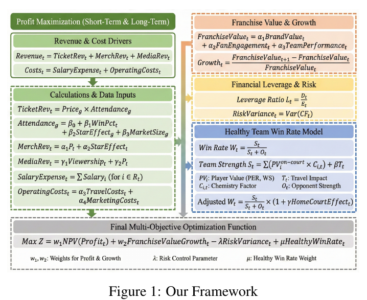
The full framework combines short-term profit, competitive performance, franchise growth, and financial risk. Four linked modules apply the shared objective to roster construction, expansion, pricing, and injury response.
A shared objective with hard constraints
The base model maximizes a weighted utility with four components: discounted profit, franchise-value growth, healthy win expectation, and a penalty for financial risk. Revenue includes ticket, merchandise, and media channels; costs include salary, travel, operations, and marketing. Competitive strength depends on player value, lineup effects, opponent strength, home advantage, and travel-related fatigue.
The objective is evaluated only inside a feasible roster region. The model enforces an 11- or 12-player roster, minimum guard, forward, and center coverage, individual salary bounds, an operating budget, and the WNBA salary-cap assumption used in the report. These constraints matter because an attractive player combination is not useful if it cannot be registered or paid for.
The four later modules are not independent stories. Expansion changes travel and talent scarcity; pricing turns expected demand into revenue; injury changes both team strength and the star effect. All of them feed back into the same competitive-financial objective.
Turning public records into model inputs
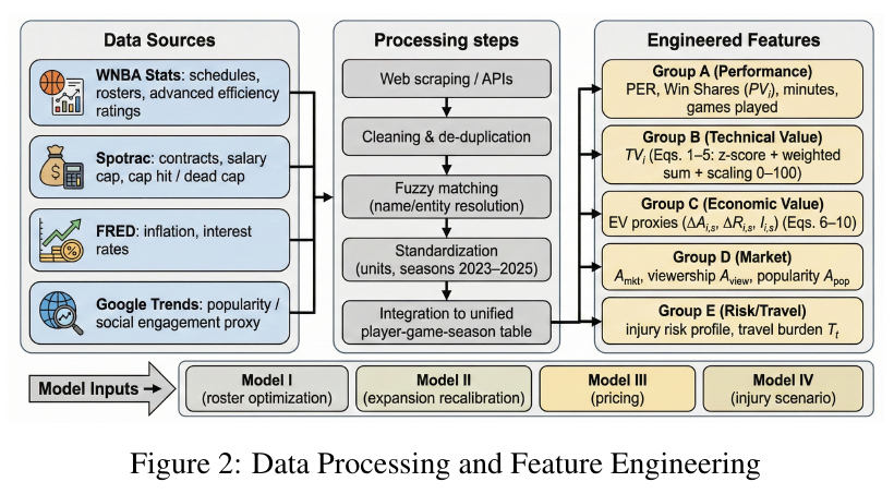
The data pipeline joins basketball performance, contracts, macroeconomic context, and attention proxies before producing a unified player-game-season table for all four models.
The project combines schedules, rosters, game logs, efficiency ratings, contracts, cap reports, inflation and interest-rate context, popularity, and social-attention proxies. Sources include WNBA Stats, Spotrac-style contract records, FRED, and Google Trends. Web-scraped and API records are cleaned, de-duplicated, fuzzy-matched across naming conventions, and normalized across the 2023-2025 seasons.
Player evidence is divided into several roles:
- Performance inputs summarize efficiency, win contribution, playing time, and availability.
- Technical value (TV) standardizes basketball metrics within each season, applies fixed weights, and scales the result to a 0-100 index.
- Economic value (EV) uses within-season home attendance and occupancy differences between games in which a player appeared and games in which the player did not appear.
- Market inputs represent viewership, popularity, and market size.
- Risk inputs summarize injury exposure, schedule density, and travel burden.
The economic-value variables are correlation-based proxies. They can help organize market evidence, but they do not prove that one player’s appearance caused the observed attendance difference.
Seeing player value in two dimensions
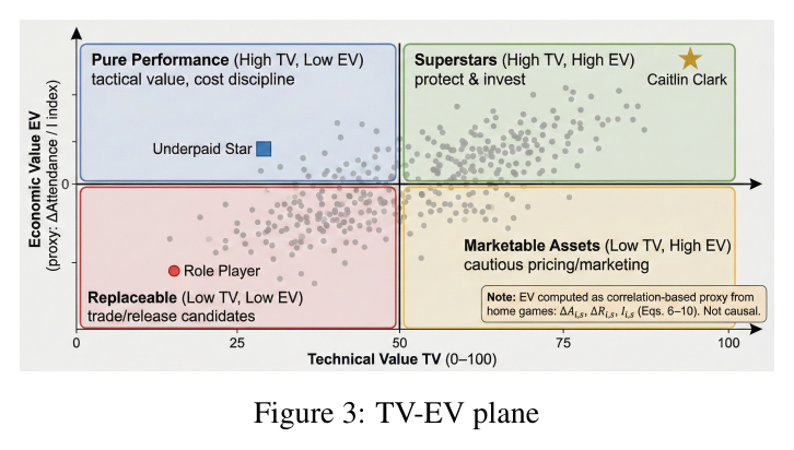
The TV-EV plane separates on-court contribution from attendance and attention proxies. The quadrants support different actions: retain and invest, protect underpriced talent, market cautiously, or consider replacement.
A single performance score cannot express every management tradeoff. The two-axis value map therefore distinguishes four broad player profiles:
- high TV and high EV: core assets to protect and invest in;
- high TV and lower EV: potentially underpriced basketball value;
- lower TV and high EV: marketable assets that require cost discipline;
- low TV and low EV: candidates for replacement, trade, or release.
This segmentation supplies interpretable inputs to the roster optimizer. It does not automate a final transaction decision, because contract guarantees, negotiation feasibility, team chemistry, and future development remain only partially modeled.
Model I: constructing a feasible 2026 roster
Player retention, signing, release, and draft choices create a mixed discrete and nonlinear search problem. The project uses Differential Evolution with threshold decoding: a continuous candidate vector is converted into binary roster decisions, while a large penalty rejects violations of the salary cap, roster size, positional balance, or draft logic.
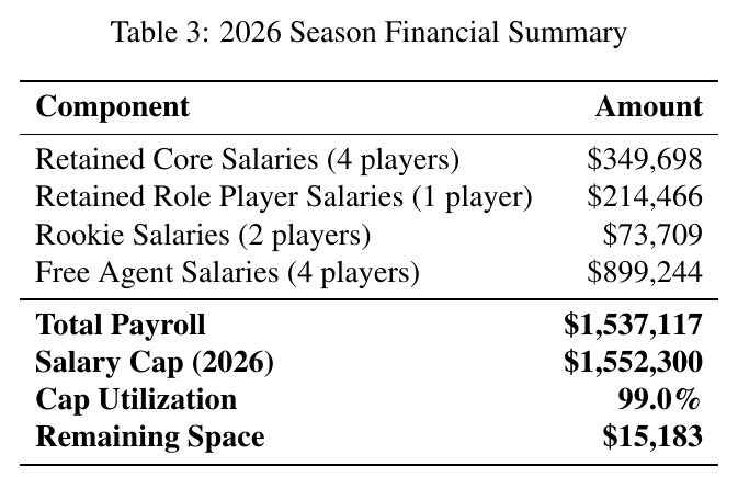
The original financial summary reports the modeled roster payroll, salary cap, utilization rate, and remaining emergency space.
Under the report assumptions, the solver identifies five low-efficiency or high-cap-pressure contracts and clears $546,231. It then combines retained players, four modeled free-agent additions, and two low-cost rookies. The final 11-player roster has a modeled payroll of $1,537,117 against a $1,552,300 cap, corresponding to 99.0% utilization and a $15,183 buffer. The projected win rate is approximately 0.545.
I treated this roster as a scenario output for the competition problem. Real availability, negotiations, team preferences, and later information were outside the model.
Model II: adapting when the league expands
League expansion affects more than the number of opponents. New West Coast and international travel changes fatigue and operations; expansion drafts dilute the talent pool; new markets create attention opportunities; and unfamiliar revenue sharing increases uncertainty.
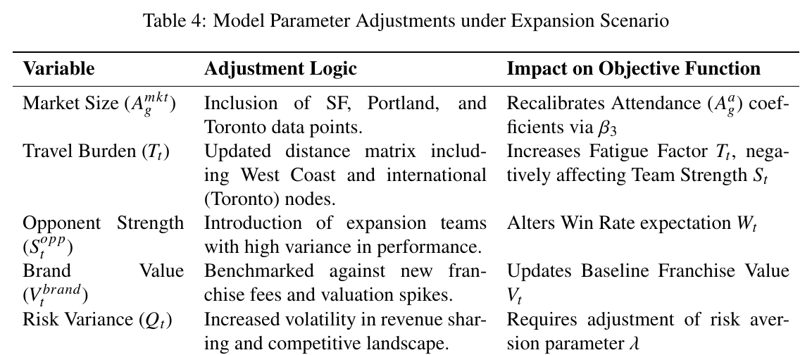
The original expansion table records how market size, travel burden, opponent strength, franchise value, and risk variance are recalibrated in the model.
The expansion version of the model moves from peak roster efficiency toward robustness. It favors the 12-player upper bound to absorb travel, prioritizes centers and multi-position frontcourt players, increases the marginal value of cost-controlled rookies, and avoids long guarantees for non-core players. It also treats inefficient salary as an asset-conversion opportunity rather than simply a sunk cost.
The main lesson is structural: the best roster under a stable league is not necessarily the best roster under a travel and talent-scarcity shock. A decision model should be recalibrated when the environment changes instead of reusing a previously optimal solution unchanged.
Model III: pricing from demand signals, not intuition alone
The base revenue equation would be unrealistic if ticket prices could rise without reducing attendance. The pricing module therefore introduces a demand-response function, venue capacity, four game-demand tiers, seat-zone multipliers, and four pregame update windows: D-45, D-21, D-7, and D-2.
At each window, two observable signals define the decision state. The sales pace ratio compares actual inventory clearance with a target curve. The secondary price index compares resale and primary-market prices. Together they determine whether the team should discount, bundle, hold price, release more inventory, or protect yield.
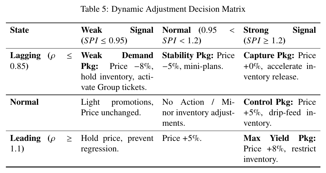
The matrix translates internal sales pace and external resale signals into nine operational packages. Price changes remain inside guardrails, and weak demand can trigger product bundles instead of repeated discounting.
The model restricts realized prices to 70%-130% of the season-ticket-equivalent anchor. Strong demand can justify controlled price increases or slower inventory release. Weak demand can trigger mini-plans, group tickets, family packs, or value-added bundles. VIP inventory is managed more conservatively than upper-tier seats to avoid eroding the long-term price anchor.
This module is designed as a feedback loop: if a price action does not restore sales pace, the strategy switches from price changes to product and inventory actions.
Model IV: responding to a key-player injury
The final module studies a severe second-half absence scenario for a core player. The shock propagates through two paths. Removing player value reduces modeled team strength and win expectation; removing the star effect lowers expected home demand.
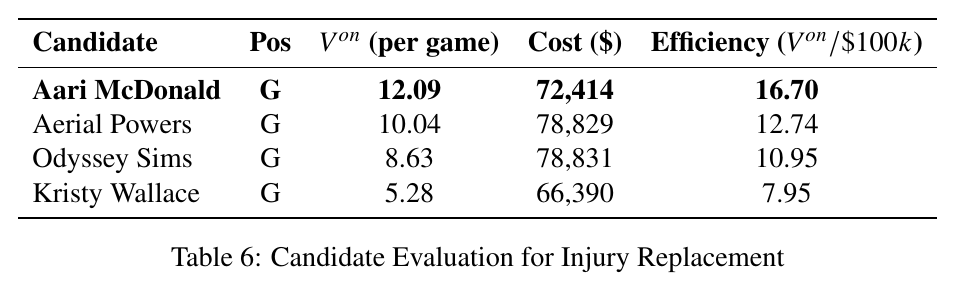
The original replacement table compares candidate player value, cost, and value-to-cost efficiency for the injury scenario.
The report estimates a win-rate decline of approximately 0.035-0.060 and an attendance decline of roughly 3,280-3,480 spectators per home game under its fixed coefficients. A replacement screen compares available guards by modeled value per $100,000 of cost; Aari McDonald ranks first in the scenario with an efficiency value of 16.70.
Signing a replacement is only one part of the response. The modeled plan also redistributes ball handling and scoring, emphasizes high-low interior play, moves marketing from a star-centered narrative toward team value, activates lower-tier bundles, and increases the liquidity buffer for higher cash-flow volatility.
What the sensitivity analysis changes
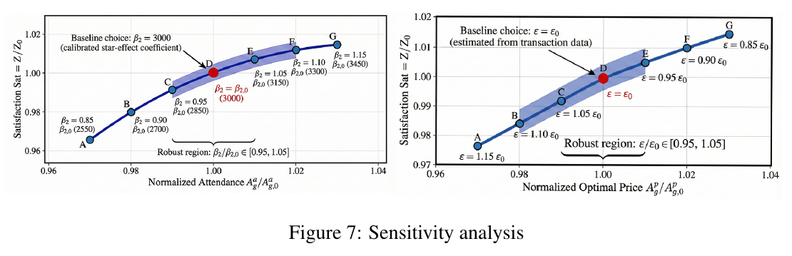
A one-factor-at-a-time test perturbs the star-effect and price-elasticity coefficients by plus or minus 15%. The objective is more exposed to star availability than to moderate pricing-estimation error.
The star-effect coefficient is the larger fragility. It directly changes attendance and ticket revenue, so underestimating or overestimating it materially changes the integrated objective. This supports minutes management, medical contingency planning, and maintaining replacement flexibility.
The pricing module is comparatively stable. Moderate elasticity changes alter the preferred price, but the overall objective moves only a few percent because price guardrails and inventory actions prevent extreme solutions. This is a useful distinction: not every uncertain parameter deserves the same amount of management attention.
What I learned from the project
The main lesson for me was that a broad management prompt becomes easier to reason about when the data definitions, constraints, and scenarios share one structure. I also learned that an optimization result is only useful when its feasibility conditions and sensitivity to uncertain parameters are visible.
Its limitations are equally important:
- revenue relationships are largely linear and omit market saturation;
- player contributions and chemistry are simplified into additive terms;
- opponent behavior is treated as relatively static;
- travel fatigue is deterministic and does not represent individual physiology;
- the main optimization is a single-season model rather than a multi-stage contract and draft-capital program;
- attendance-based EV and scenario coefficients are modeling proxies, not causal estimates or forecasts.
If I continued the project, I would add multi-period stochastic optimization, richer lineup interactions, contract-option logic, and uncertainty intervals for demand. I present the current version as a completed undergraduate modeling competition project and a record of my work with data integration, optimization, and scenario analysis.