What I worked on
NSOFC-RegRank was my main computational research project to date. I worked on turning heterogeneous GWAS records into a traceable candidate-variant workflow: organizing source data, harmonizing coordinates, checking allele fields, adding regulatory annotations, and comparing model outputs without hiding missing coverage.
The biological setting made the data work challenging. Genome-wide association studies can identify loci associated with nonsyndromic orofacial clefts (NSOFC), but a lead variant is rarely the complete explanation. Nearby variants may be correlated through linkage disequilibrium (LD), most candidates are noncoding, and a regulatory effect may depend on tissue and developmental stage.
The project therefore focused on a practical question: within a GWAS locus, which candidates have enough supporting evidence to be considered earlier for functional follow-up? I treated the output as an organized set of hypotheses for later experiments, not as a diagnosis or a list of confirmed causal variants.
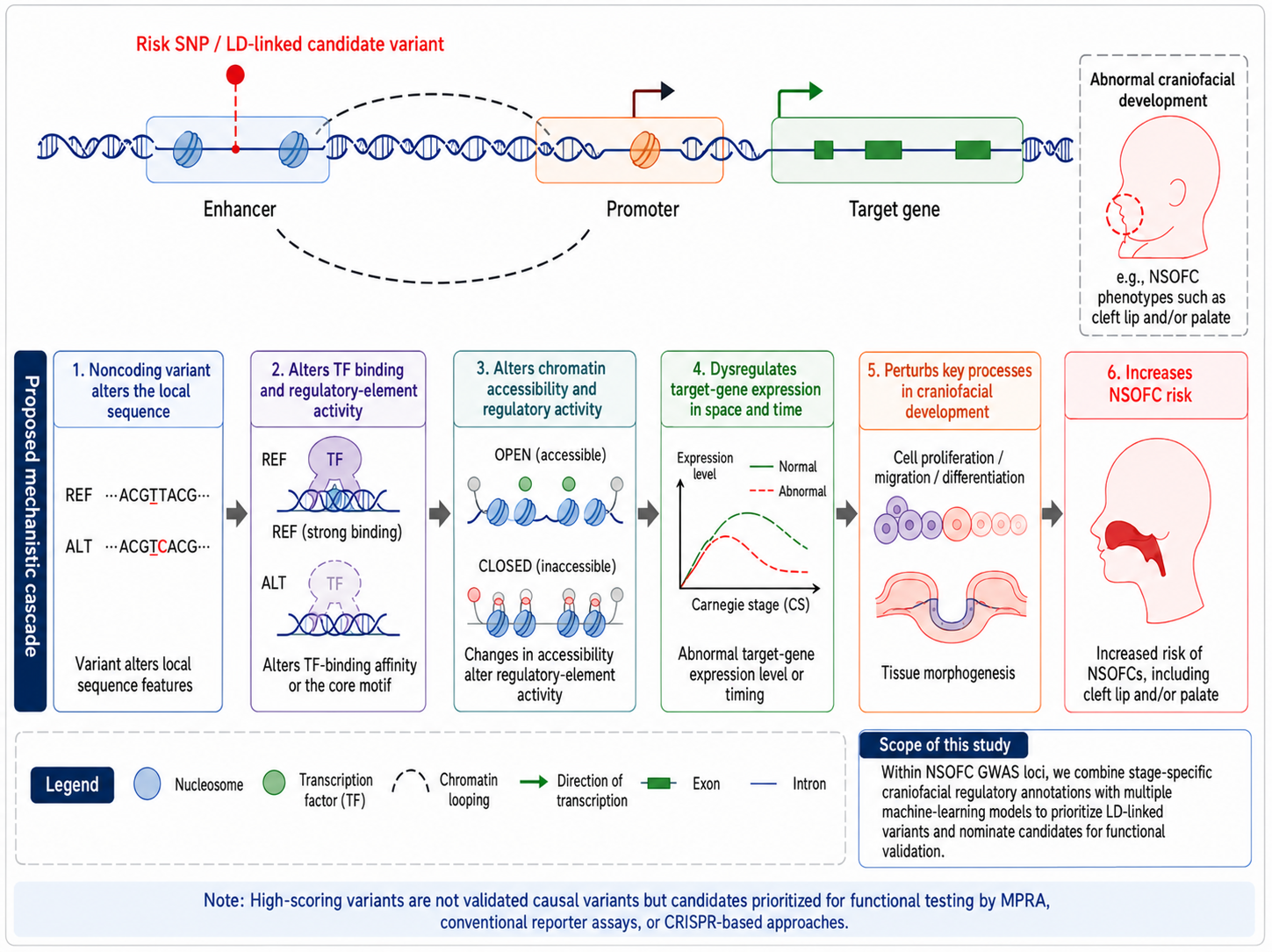
The mechanism chain gives the biological context for prioritization: a noncoding sequence change may affect transcription-factor binding, chromatin accessibility, target-gene expression, and craniofacial development.
How I organized the workflow
I organized the workflow from GWAS source records to locus-level candidate summaries. My main goal was to make each transformation traceable, especially the coordinate, allele, provenance, and model-coverage fields that are easy to lose during data cleaning.
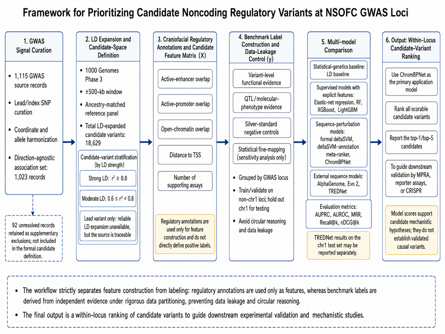
The pipeline separates source curation, LD expansion, craniofacial annotation, benchmark construction, model screening, coverage checks, and validation-oriented outputs.
The main stages are:
- GWAS source curation. Phenotype names, study accessions, lead variants, reported alleles, effect directions, and genome builds are normalized without pretending that missing direction information is known.
- Coordinate and allele auditing. Records are aligned to hg19/GRCh37, rsIDs are reconciled, and REF/ALT fields are checked against the reference sequence. Strand ambiguity and symbolic or imprecise alleles are retained as explicit states rather than silently coerced.
- LD candidate construction. Ancestry-matched 1000 Genomes references define locus-level candidate spaces. LD expansion describes correlation with an association signal; it does not prove functional mediation.
- Craniofacial regulatory annotation. Candidates are intersected with promoters, enhancers, open chromatin, MPRA evidence, expression support, and craniofacial-relevant resources after coordinate harmonization.
- Benchmark and model evaluation. Transparent genetic and regulatory baselines are compared with supervised pilot models and external sequence-based scores under explicit label and coverage constraints.
- Validation hypothesis generation. Ranked candidates are reported with their evidence domains, missingness, locus denominator, and suitable follow-up experiments.
The report snapshot contains 22,739 main candidate variants across 14 functional loci. Those counts define the primary denominator. Smaller subsets are used only when a model can validly score every required candidate or locus.
What sparse labels taught me
Functional positives are scarce, heterogeneous, and usually concentrated in a small number of well-studied loci. More importantly, an unlabeled candidate is not a biological negative. It may simply never have been tested.
This was one of the most important statistical lessons from the project. Treating every unlabeled variant as negative would create label noise and could reward a model for reproducing historical study bias. I therefore kept strict positives, silver-standard positives, lower-evidence controls used for pilot analysis, and unlabeled candidates as distinct groups.
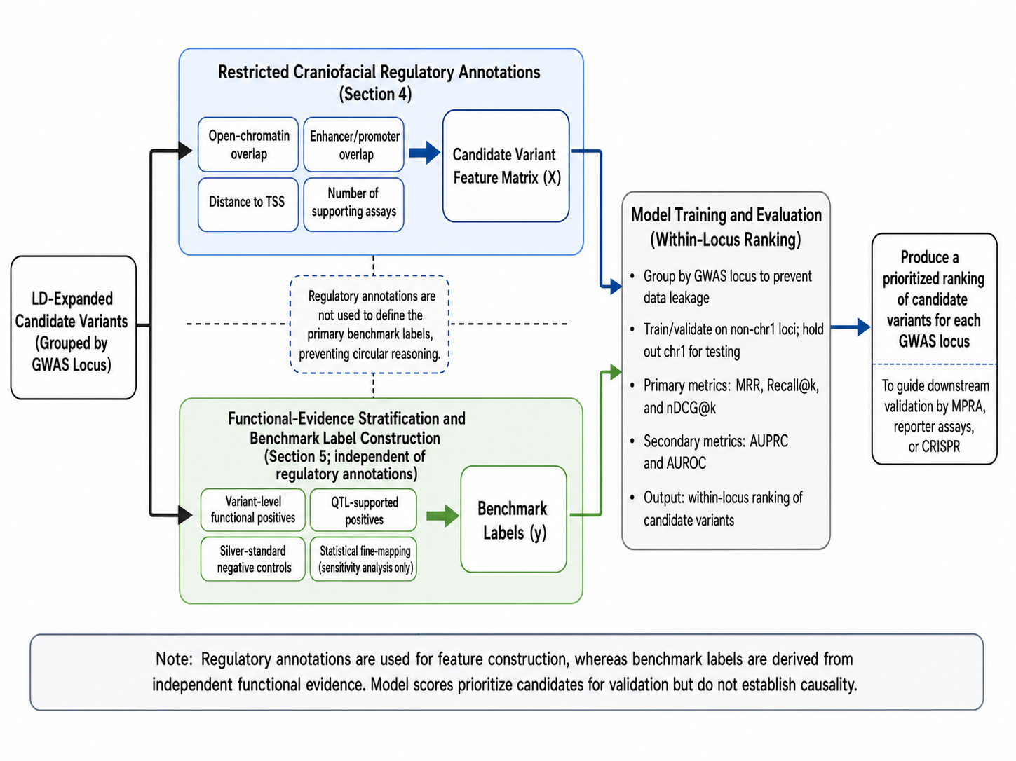
The figure shows the main leakage-control rule: regulatory annotations used as features are kept separate from the evidence used to define benchmark labels.
The separation matters because a model should not be evaluated on a label that was directly constructed from the same annotation it receives as input. Feature definitions and benchmark evidence are therefore audited by source and role. Locus-aware splits and within-locus ranking metrics are preferred over random variant-level accuracy.
Starting with simple baselines
Before interpreting machine-learning scores, I compared them with simpler references: LD strength, distance to the lead variant, distance to transcription start sites, regulatory overlap, and a weighted annotation score. This helped me ask whether a complex model added useful ranking information beyond common genetic and annotation heuristics.
Traditional supervised models, including elastic-net, random forest, XGBoost, LightGBM classification, and a LightGBM ranker, are used in a chromosome 1 pilot analysis. Their purpose is to test whether the available tabular features contain an initial ranking signal and to expose instability caused by the small effective positive denominator. They are treated as screening and sensitivity evidence, not as the main disease-specific ranking result.
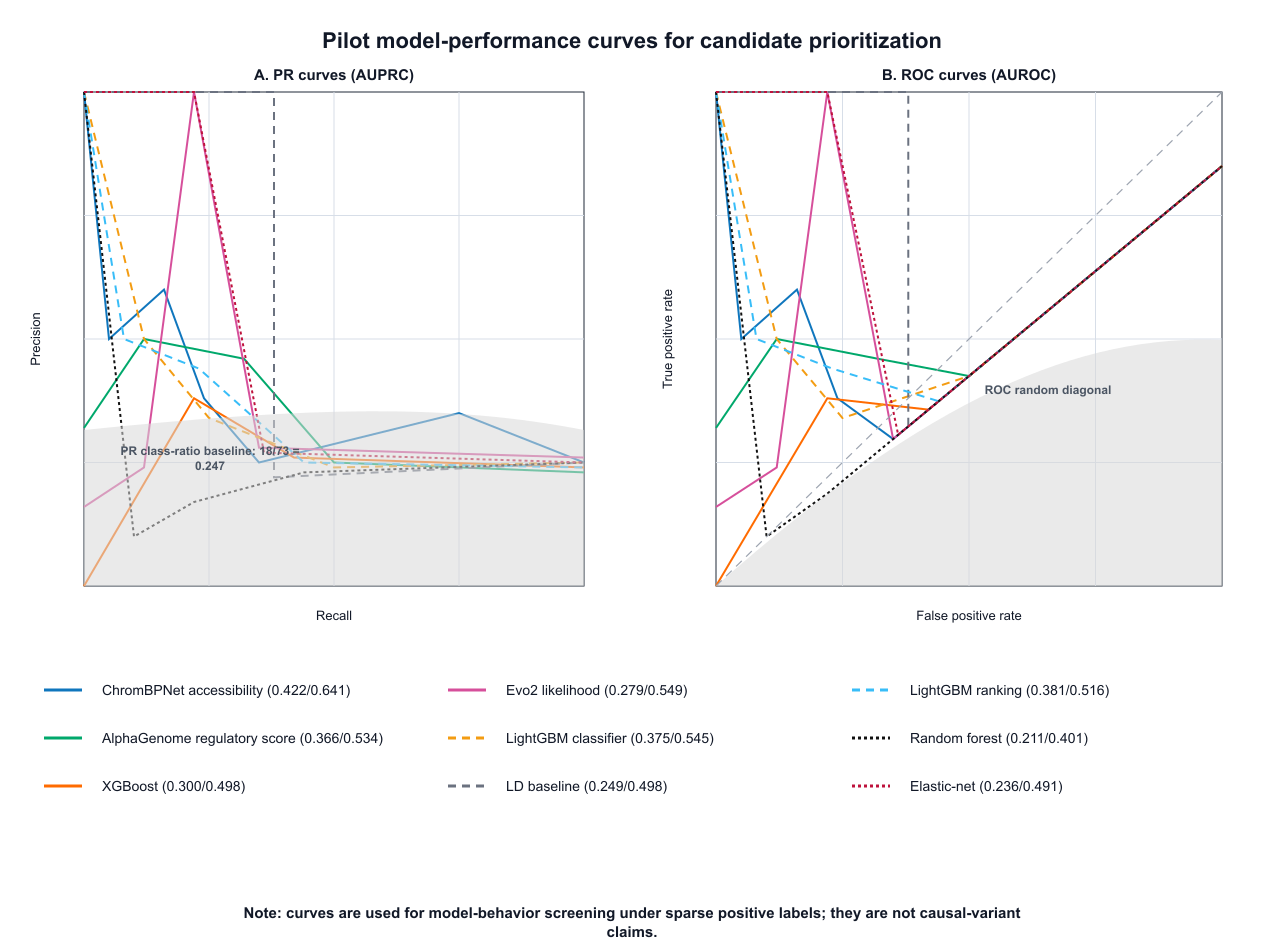
The PR and ROC curves summarize pilot screening behavior under sparse positives and substantial class imbalance.
Comparing external models carefully
ChromBPNet, AlphaGenome, and Evo2 provide different sequence-based signals. ChromBPNet is related to sequence effects on chromatin accessibility, AlphaGenome provides broader sequence-to-function predictions, and Evo2 contributes a general sequence-likelihood perturbation score. Their outputs are not interchangeable biological quantities.
Before comparison, I checked whether the runtime was reproducible, REF and ALT sequences were valid, score direction was documented, and locus coverage was complete. I kept unscored variants as missing rather than turning them into zeros.
Only 10 of the 14 primary loci currently form a common complete-coverage subset for the three external models. That subset supports a secondary descriptive triage analysis. The remaining four loci stay in the 14-locus benchmark through transparent baselines and coverage auditing. In the report snapshot, strict positives cover only 20 of 64 positive records within the common external-model subset, which further limits interpretation.
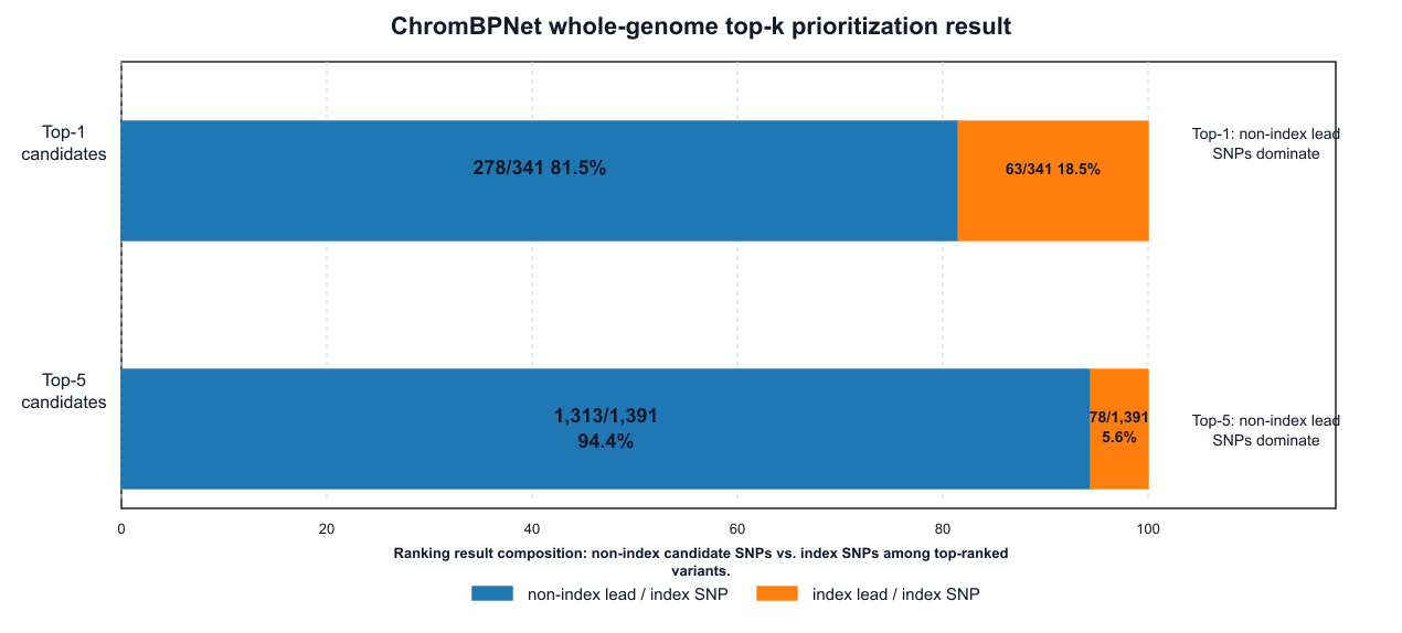
The top-k view asks whether known functional positives appear near the top of ranked locus-level candidate lists within the eligible subset.
The current comparison suggests that AlphaGenome’s descriptive retrieval point estimate is closer to the weighted regulatory baseline, while ChromBPNet and Evo2 do not show the same top-rank retrieval signal in this small common-coverage subset. Because the denominator is only 10 loci and positive coverage is incomplete, this observation remains secondary and descriptive.
From scores to follow-up ideas
Candidate nomination follows evidence tiers. The strongest hypotheses combine support from a transparent baseline and one or more external models within a completely covered locus. Candidates supported only by the 14-locus transparent baseline remain valid hypotheses but are labeled accordingly. Literature-prioritized candidates with incomplete model coverage enter an audit pathway rather than being dropped.
Each candidate record should report its locus, candidate count, LD and distance context, regulatory evidence, model score and coverage status, benchmark label if available, and an appropriate experimental next step. Missing fields remain missing. This is important because a polished ranking without visible missingness can appear more certain than the underlying evidence permits.
What I learned and the project limits
The largest limits are the incomplete craniofacial regulatory maps, the small number of experimentally supported positives, and the 10-locus common-coverage subset available for the external-model comparison. These constraints mean that the ranking is most useful as a way to organize evidence and choose follow-up candidates.
For me, the main value of the project was learning how data definitions, missingness, label construction, and evaluation denominators can change a modeling result before the choice of algorithm even begins. It also gave me practical experience with Python, R, shell workflows, genomic data formats, model-output aggregation, and technical documentation.
I now consider the computational project complete. The resulting candidate records and workflow are a record of my research training; any biological conclusion would still require experimental validation.